30) Using VLOOKUP (or HLOOKUP) in Microsoft Excel

VLOOKUP is a very useful formula in Excel to perform tasks such as:

• Data comparions between sheets
• Checking for discrepancies
• Linking data between sheets

and the list can go on!

The formula looks like this:
VLOOKUP(lookup_value,table_array,col_index_num,range_lookup)

--
lookup_value: The value to search in the first column of the table array

table_array: Two or more columns of data. The values in the first column of table_array are the values searched by lookup_value. These values can be text, numbers, or logical values. Uppercase and lowercase text is equivalent.

col_index_num: The column number in table_array from which the matching value must be returned. A col_index_num of 1 returns the value in the first column in table_array; a col_index_num of 2 returns the value in the second column in table_array, and so on. If col_index_num is:

• Less than 1, VLOOKUP returns the #VALUE! error value.
• Greater than the number of columns in table_array, VLOOKUP returns the #REF! error value.

range_lookup: A logical value that specifies whether you want VLOOKUP to find an exact match or an approximate match:

• If FALSE, VLOOKUP will only find an exact match. In this case, the values in the first column of table_array do not need to be sorted. If there are two or more values in the first column of table_array that match the lookup_value, the first value found is used. If an exact match is not found, the error value #N/A is returned.

• If TRUE or omitted, an exact or approximate match is returned. If an exact match is not found, the next largest value that is less than lookup_value is returned.

--

The values in the first column of table_array must be placed in ascending sort order; otherwise, VLOOKUP may not give the correct value. You can put the values in ascending order by choosing the Sort command from the Data menu and selecting Ascending. For more information, see Default sort orders.

A good reference for more details of the formula can be found here.
These details are illustrated in the following example.

Step 1:
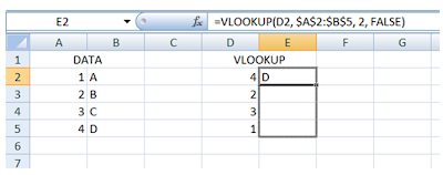
a) Once you have your table_array (i.e. your “reference dataset” with the first column containing), and the list which you would like to lookup for, enter the VLOOKUP formula in the cell as follows:

b) Note that in the formula, I have put in a “$” sign for the data source table indexes. This is to lock the table_array as A2:B5 and not allow it to slide as we drag the formula down to the rest of the cells.
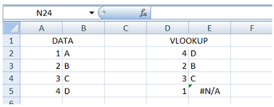
This is what it’ll look like if I had not put the “$” sign there:

Notice that the data source table_array indexes have shifted (green box) and hence the value “1” could not be found. This will result in a #N/A error, as follows:

To avoid this, it is safer to use the “$” sign in your formula as shown in the Step 1(a).

Step 2: Hover on the edge of the cell, till your cursor becomes a “+”.
Click and drag the formula down to fill the rest of the cells.


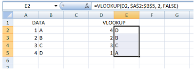
Step 3: And this is what you’ll get:

For data comparions from different sheets:
If your source/reference data is stored in another sheet, simply add the sheet name at the beginning of the [table_array] field, like this:

What if I have a horizontal set of data as my table_array?
The VLOOKUP formula described above is used when the table_array is vertical and the lookup values are in the first column.
Use HLOOKUP when the table_array is horizontal and the lookup values are in the top row. The other details, such as using the “$” sign, remain the same.

What does #N/A mean?
The error #N/A indicates that the source for a particular data was not found in the table_array. This could mean either (i) your table_array had shifted, as explained above in Step 1(b) or (ii) the data of interest is not present in the reference table.

Counting the #N/A's
Sometimes we might be interested in the number of data entries that do not have a match in the table_array (the reference table).

To count the number of #N/A errors in a dataset, use this formula:

=IF(ISNA(A1),1,0)

This prints 1 if cell "A1" contains #N/A, else prints 0. Sum up the column to obtain a total.